Services with high-performance computing Services with high-performance computing
 |
|
<Related information> High-Performance Computing on Cloud Services (Up&Coming '11 Fresh Green Issue)
| LuxRender Rendering Service NEW! |
|
|
|
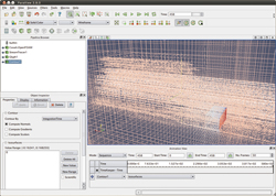
LuxRender
is a one of the many types of software collectively called the
"renderer" which performs image processing based on 3DCG models
created. The images are created by performing shading, etc. based on
each of the different types of information concerning the created model
such as its view point and light source. Among these renderers,
LuxRender stands out as is good at physically calculating the behavior of lights very accurately to give you a realistic image like a photograph.
Due to its nature, LuxRender does not have a concept of ending a rendering,
thus the operator can assign the rendering time at will. As rendering quality
increases the more you spend time on it, rendering time is decided by looking
at the balance of quality and cost.
About LuxRender Rendering Service
|
In this service, still images and videos are created by performing rendering
using LuxRender based on the scenes received by 3dsMax. The work flow of the service
is as follows.
- Checking the scene content
- Cost estimation
- Create rendering sample
- Signing a contract
- Determining the level of quality
- Rendering
- Review
- Delivery
First, we will investigate whether the received scene can be rendered via LuxRender (step 1).
If it is ascertained that rendering is possible, we will move to cost estimation (step 2).
After estimating the cost, we will move to the stage in which a rendering sample image is created (step 3).
In this step, we will actually render the received scene via LuxRender,
but this is still at a preview stage. Material conversion is
a very simple one and the rendered image will be a small one that can be created
in a short time. The client will have an idea an image of the finished product
here. If we can obtain the client's agreement on the created sample image,
we move on to the contract phase (step 4).
Rendering quality is decided after the contract is made (step 5).
Based on the image created in step 3, things that need to be adjusted or corrected within the entire scene such materials which can be assigned either automatically or by hand, and lighting are determined.
When the rendering quality is decided, the main rendering is carried
out after the revision of the received scene accoriding to the level of quality decided
(step 6).
Review is done based on the image obtained by this main rendering (step 7).
If the client asks for quality improvement in the review phase, then
the
contract is renewed and the contents within the scene that need to be
corrected and
additional rendering time is determined. After the scene has
been corrected, the review of the rendered image and the result is
done again.
The work flow from the contract phase to the review phase is repeated
until the client is
satisfied with the quality. We move on the the delivery phase when the
client is satisfied with the quality. A figure showing the work flow of
the service is presented on the right.
|
| Quality level determination |
Review
*repeat from making a contract to reviewing |
|
 The work flow of service The work flow of service |
|
|
Automatically
converts Standard materials, which are included in dsMax by default,
into materials for LuxRender. Also, as for any of the map channels such
as diffuse reflection light color, specular reflection light color,
bump, and displacement, bitmap and mixmap designed in these channels
are automatically converted for LuxRender.
The material textures
that could not be converted in the scene are manually converted. (Those
failing in conversion are output as a list in a text file.)
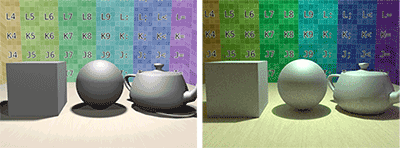
Comparison of the standard material with LuxRender material when each is rendered to an image is shown below.
●Materials without luster
 |
Comparison when materials are without luster
Left : Standard material, Right:LuxRender material |
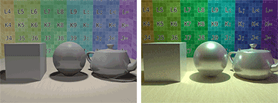
●Materials with luster, and can also express reflection
・without reflection
 |
Comparison of materials with luster, and can also express reflection
(without reflection)
Left : Standard material, Right : LuxRender material |
・with reflection
 |
Comparison of materials with luster, and can also express reflection
(with reflection)
Left : Standard material, Right : LuxRender material |
●Materials expressing transparency
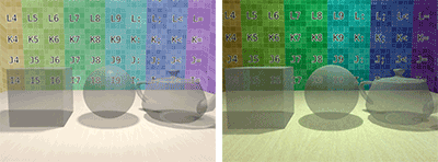 |
Comparison of materials expressing transparency
Left : Standard material, Right : LuxRender material |
●Materials expressing transparency
Presents
the conversion process when material converter script is applied to a
3dsMax scene containing an object in which a standard material is assigned.
If a converter script is run, it first examines the objects in the scene. It
checks whether a material is set for each object and examines the type
of material if this is the case. If the type of material is a Standard
material normally attached to 3dsMax, it automatically chooses a type of
material for LuxRender from various parameters and applies it. If the material
set to the object is a Standard material, the material is placed as it
is. In this case, it will be converted manually.
For the Standard materials which have been automatically converted, an
automatic conversion of textures will be performed in the next step. 2
conditions are judged at the phase of converting the texture, and
automatic conversion is done if it meets both conditions.
The first condition is the type of texture. The type of texture must be
either "Bitmap" or "Mixmap".
The second condition is the channels in which the texture is set. Those channels
must be either of "Diffuse reflection light color", "Specular
reflection light color", "Bump", or "Displacement".
The assigned texture is converted into a texture for LuxRender when these
two conditions are met. On the one hand, the texture conversion is done
manually in a case when the conditions cannot be met. |
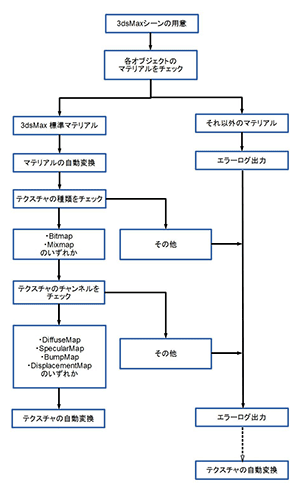
Conversion process |
|
<Related information> High-performance computing on cloud services (Up&Coming '11 Fresh Green Issue)
 Engineer's Studio® High-performance computing on cloud services option Engineer's Studio® High-performance computing on cloud services option |
Released on 2011/08/24 |
|
Engineer's Studio® is an analysis program with Finite Element Method(FEM), developed in-house
from pre-processing, calculation engine, to post-processing. This program
allows various analysis including static analysis, dynamic analysis, and
eigen value analysis. It supports for material nonlinear models and geometric
nonlinear models. The structural analysis using beam elements, fiber elements,
and plate elements can be performed.
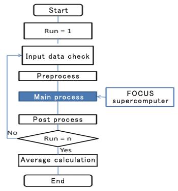
For this time, we have launched "Engineer's Studio® Cloud Service"
where the main calculation is supported by FOCUS high-performance computing(*1).
This allows the scale for analysis to be enlarged and the time taken for
analysis to be reduced in Engineer's Studio®. In this service, the
data is automatically linked with FOCUS high-performance computing by creating
and registering them via the Internet. The final result data is scheduled
to be taken via web application, saved in a medium and sent to the customers
according to the situation. |

 |
|
 |
|
|
|
|
Figure1 Process image of Engineer's Studio®analysis service |
Analysis method of high-performance computing on cloud services option
|
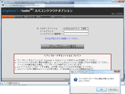
1.Create and save the input data with Engineer's Studio®. |
|
2. Log-in the UC-1 for SaaS server. |
|
3. Upload the input data.(Input the job) |
|
|
 |
 |
 |
|
 |
|
|
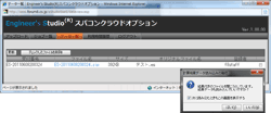
4. Download the analysis result. |
|
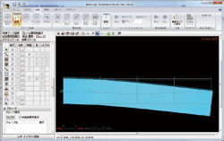
5. Display the result, and create the report with Engineer's Studio®. |
|
 |
|
 |
|
Future development
- Parallelization for multiple nodes
- Added option for selecting the result data before analysis to get only
the required data from a number of analysis data.
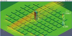
| High-performance computing option, Analysis support service |
This service is an option of the existing Engineer's Studio® analysis
support service. Engineer's Studio® supports for nonlinear plate elements.
The problems such as calculation time or memory consumption are sometimes
occurred in large scale models. The high-performance computing allows the
reduction of calculation time and the improvement of analysis accuracy
by supporting precise model analysis. In the analysis of 300 seconds (30,000
steps at intervals of 1/100 seconds), which was measured in the 2011off
the Pacific coast of Tohoku Earthquake, known for "K-NET Tsukidate(MYG004)"
opened in Kyoshin network( K-NET), NIED, the computation time is reduced
using supercomputer. Moreover, as the seismic waveform which was measured
in the subsequent aftershock is also opened in that network, a number of
step analysis (More than 50,000 steps) can be rapidly performed with consideration
of effect of main shock and aftershock.
References:Kyoshin Network(K-NET), National Research Institute for Earth
Science and Disaster Prevention(NIED)(https://www.kyoshin.bosai.go.jp/kyoshin/)
 |
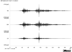 |
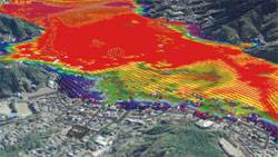
| Figure5 Maximum acceleration distribution on ground surface observed by
strong motion observation network(K-NET、KiK-net)(Left), strong-motion waveform
at K-NET Tsukidate(Right) Cited from website of NIED |
|
|
|
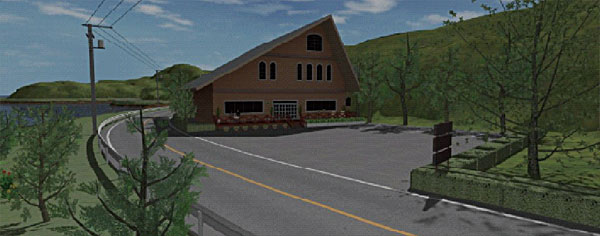
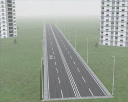
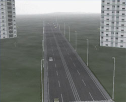
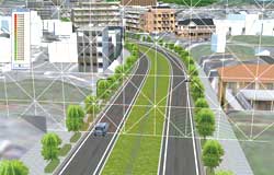
This service provides the high-accurate movie file created by POV-Ray.
The high-performance computing allows the high-accurate movie which is
not available in real. In addition, with POV-Ray, the script file can be
edited with editor after outputting with UC-win/Road.
 |
 |
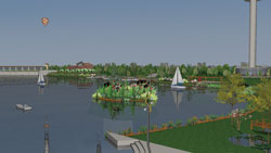 |
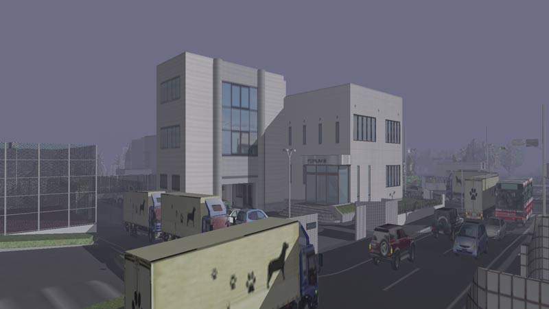
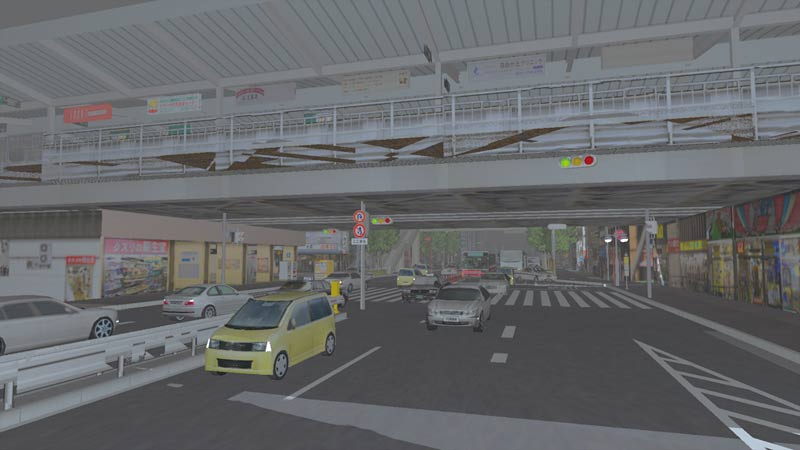
 Low number of polygons Low number of polygons
VR models of
FORUM8 Miyazaki office |
Medium number of polygons
VR model of around
Nakameguro Station, Tokyo |
High number of polygons:
Restoration VR model of
environment around
Beiyunhe, China |
- Create the scenes in UC-win/Road.
- Adjust the movie contents.
- Create the POV-Ray script.
- Render per frame(with high-performance computing)
- Create the movie file from rendered result.
- Deliver the movie file.
 |
 |
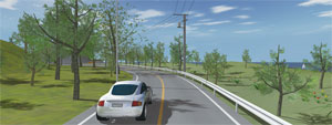 |
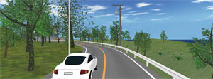
| Before rendering |
|
After rendering |
 |
| Rendering using the POV-Ray |
| 6K Digital Signage CG movie creation |
 |
UC-win/Road CG movie creation in UC-win/Road
"Driving model of a lighthouse and an island" |
| 6K Digital Signage CG movie creation |
- Supports for the creation of movie file
- Supports for the objects(Rain, snow, fire (smoke)) which were not available
for POV-Ray in Ver.5.2
 |
|
 |
| Setting of atmosphere with POV-Ray (Effect of fog) |
 |
|
|
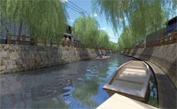
| Example of the rendered model with POV-Ray. VR model for modification of
the surrounding environment in the river, northern china. |
 |
|
 |
Model output from UC-win/Road (Left) and the rendered CG with "POV-Ray",
high-performance computer (Right) |
 |
|
 |
|
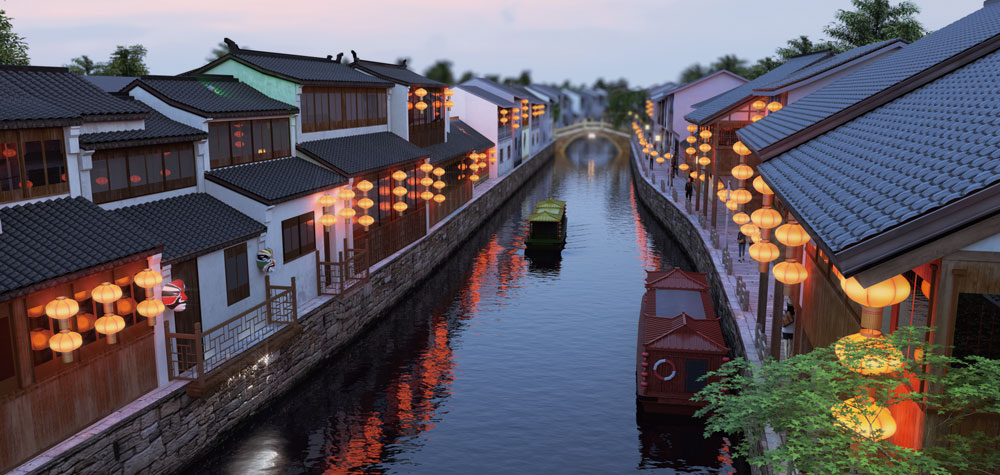
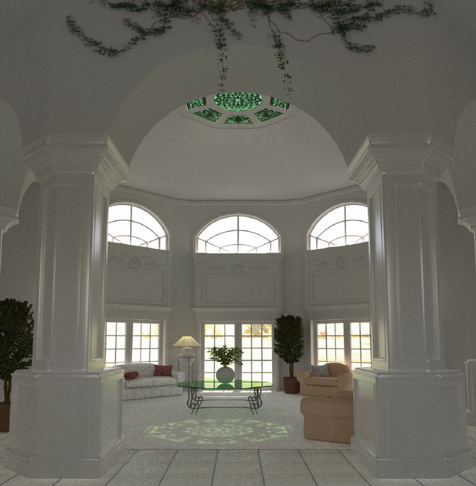
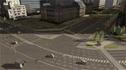
| ■ 3dsMax CG movie service |
Adoption of the trial use of K: 2013/5/17 |
This is a service providing photorealistic images often mistaken as photographs
for their extremely detailed quality, which can be generated by performing
an enormous calculation based on a real physical equation using high performance
computing of FOCUS (Foundation for Computational Science). Besides the
reviewing the design of an interior coordination of BIM models in architecture,
the service is applicable for various other purposes such as planning automobiles
and their components, reviewing a project at the design stage, presentations,
public relations, and marketing.
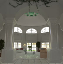 |
 |
Rendered results by 100 FOCUS
nodes within 1,000 seconds
through parallel processing |
Example of LuxRender |
|
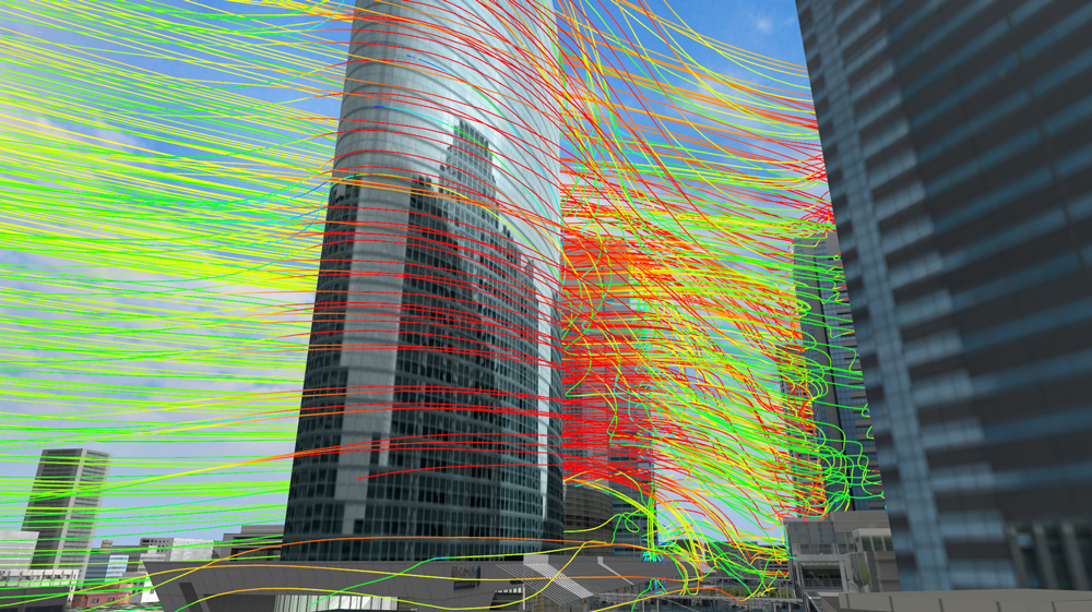
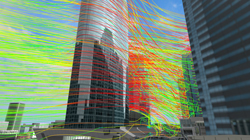
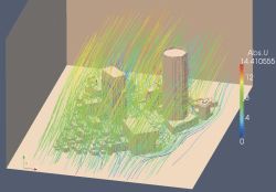
| Wind and heat fluid analysis/simulation supercomputing service |
This service is the analysis and simulation support service with general-purpose
of fluid analysis tool "OpenFOAM". "OpenFOAM" was developed
by OpenCFD and delivered with General Public License of GNU as free or
open source.It allows the simulation of complex flow including the fluid
flow with turbulent fluid and heat transfer. This service provides the
easy access to the advanced analysis environment using high-performance
computer by FORUM8's intermediate access to high-performance computer.
|
Use of current analysis part
|
- Wind analysis(Wind analysis around building)
- Water(Single fluid, fixed or free boundary)
- Multiphase fluid analysis(Gas and liquid, liquid and solid, etc)
 |
|
 |
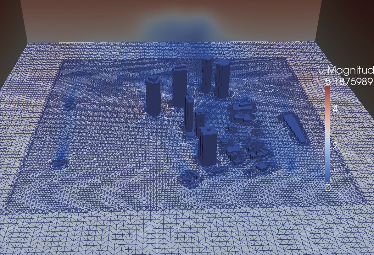
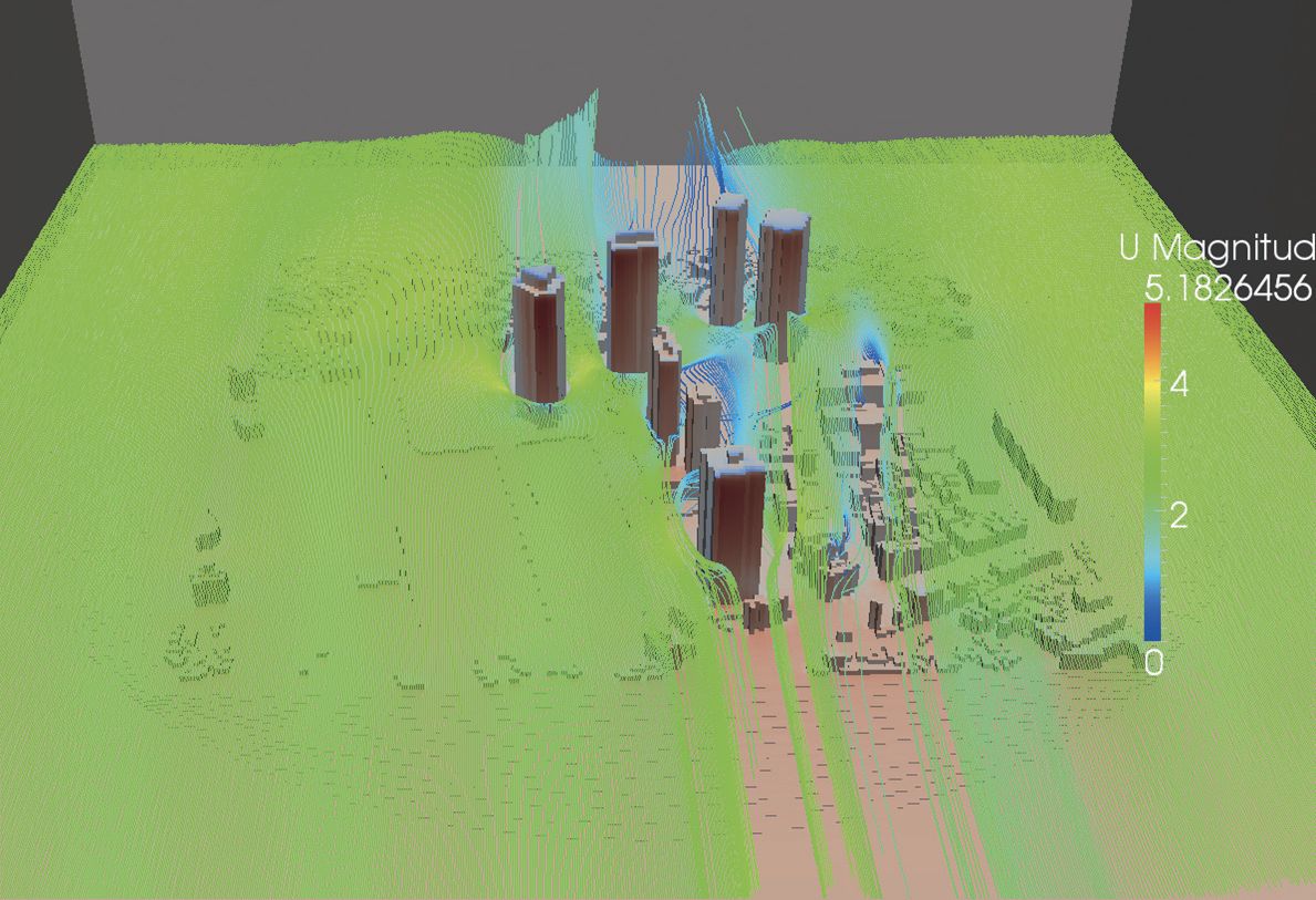
| Wind analysis with Nakameguro GT Tower model |
 |
|
 |
| Wind analysis with Shibuya model |
 |
 |
 |
|
|
Analysis example
with OpenFOAM |
 |
|
 |
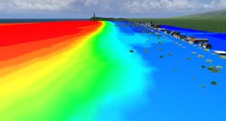
| Pressure contour diagram.The pressure and flow line per hour can be checked
by changing the time. |
 |
|
 |
 |
|
|
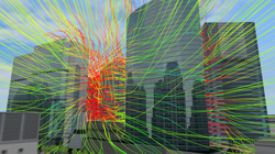
| Application example of wind analysis |
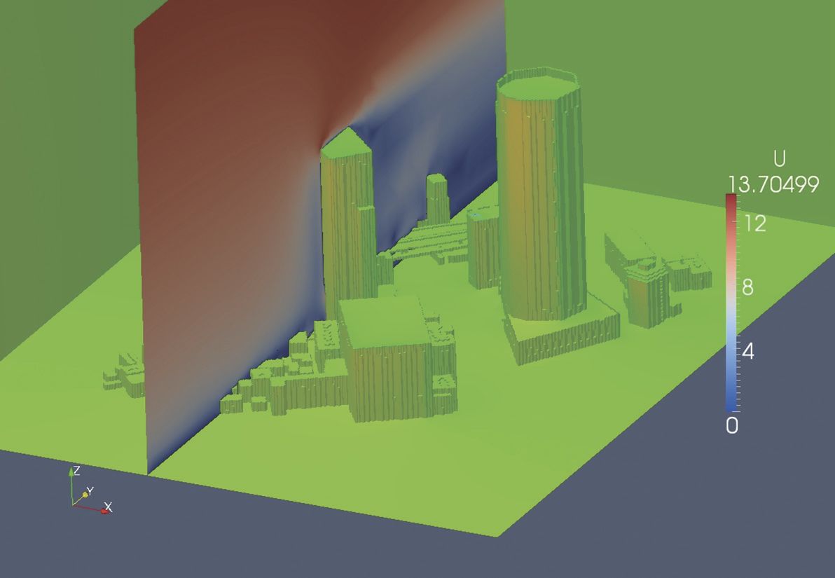
- (1) Building complex in Shinjuku, subcenter of Tokyo
Models explained in "Guidebook for Practical Applications of CFD to
Pedestrian Wind Environment around Buildings" by Architectural Institute.
The followings are the scale and overview. (Analysis time: about 2 hours
)
-Analysis range: 1700m x 1700m x 700m
-Number of node: about 750,000
-Number of element: about 1,300,000
 |
 |
Case (1) Building complex in Shinjuku,
subcenter of Tokyo: mesh and the
distribution map of wind velocity (contour) |
Case (1) Building complex in Shinjuku,
subcenter of Tokyo: the distribution map
of wind velocity (vector) |
(2) Building complex of the vicinity of Nakameguro station
Analysis example around Nakameguro station (analysis time: about 1 hour)
-Analysis range: 400m x 500m x 300m
-Number of node: about 530,000
-Number of element: about 950,000
 |
 |
Case (2) Building complex around
Nakameguro station: the distribution map
of wind velocity (vector) |
Case (2) Building complex around
Nakameguro station: the distribution map
of wind velocity (contor) |
- The base price of the service is calculated from the calculation formula
below.
| Base price |
| Direct personnel costs |
[Estimated area* Work unit* extra for shapes]* Engineer work unit cost |
| Administrative costs |
Direct personnel costs x 120% |
| General costs |
Technical costs, express charge |
The following is the price of the two model cases above.
|
Work unit |
Estimated price |
| (1)Shinjuku model |
22.2 |
¥2,162,636- |
| (2) Nakameguro model |
12.2 |
¥1,188,476- |
*Tax is not included.
- *Specific amount will be quoted separately.
|
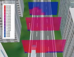
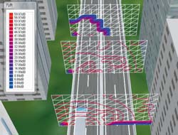
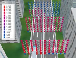
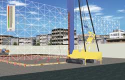
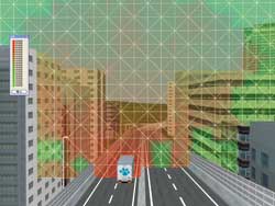
| Noise analysis/simulation supercomputing service |
Released on 2011/08/29 |
|
This service is for the simulation of noise production in general by locating
the sound source and for receiving sound in VR space.
The analysis process is performed by high-performance computer, this service
is very useful especially for the large-scaled data process.
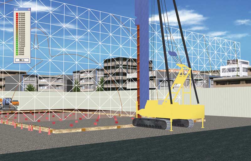
Noise Simulation option consists of Pre-processor (for data input), main
processor (for simulation) and Post-processor (for presenting result).
- Preprocessor
Data entry process of the sound source arrangement, sound receiving surface
settings, analysis condition parameters settings is performed in VR-Studio®.
- Main processor
The reflection and transmission on ground surface and model surface are
considered by setting the sound path.(The information that the judgment
of diffraction is performed described in the article of "UC-win/Road
Noise simulation option" in the previous issue is incorrect. The diffraction
is not considered.)
In the analysis process, the data can be separately processed between sound
source and sound path. The parallel computation is executed in supercomputer
using this feature to process large scale date efficiently in VR-Studio®
version.
- Post processor
Rich display options help you to capture the simulation results from various
viewpoints. In addition to contours and contour lines commonly used for
presenting the simulation results, the option also has a unique ability:
visualizing sound pressure level by grid or sphere shape.
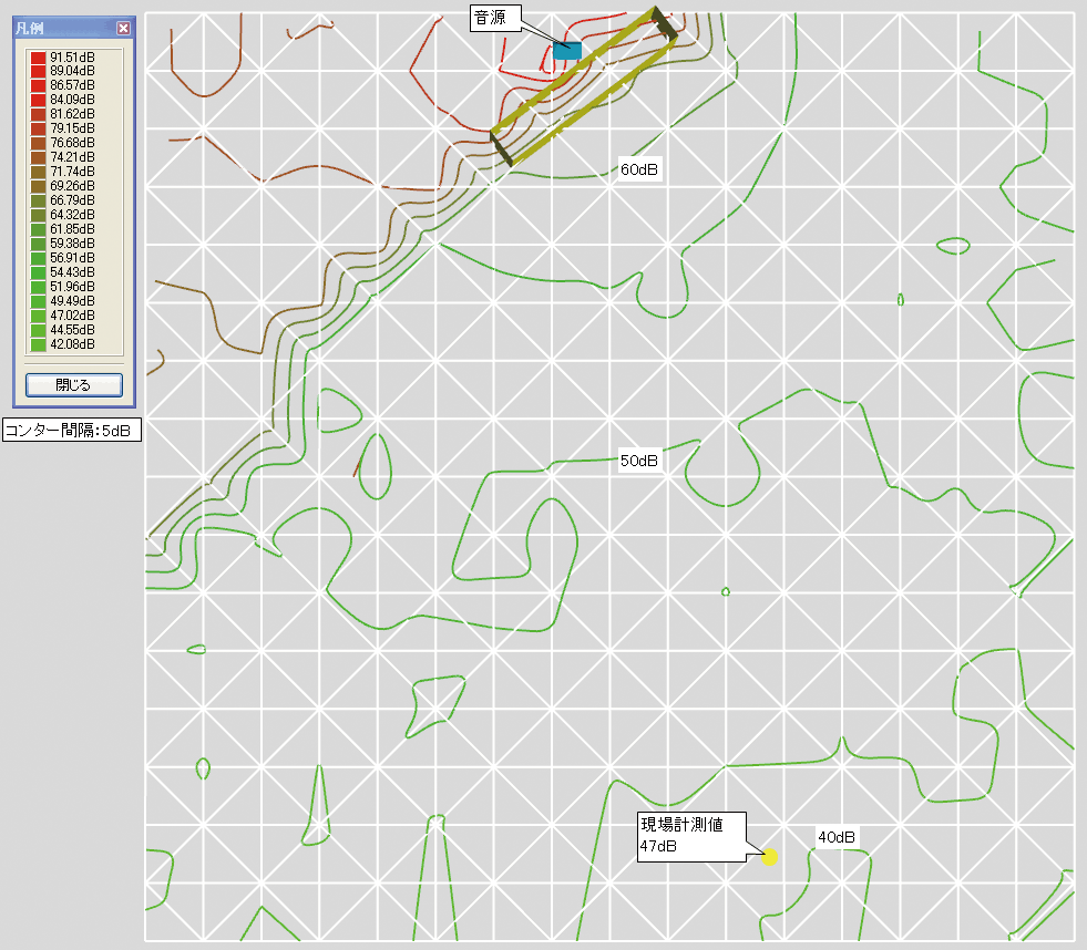
| Procedure of noise analysis |
1. Pre-process
- Import geographical data and terrain data
- Define the structures including roads and bridges
- Define the constructions including buildings
- Define the sound source and sound receiving points
- Define the analysis conditions
 |
 |
| Setting of sound source |
Placing points at once |
| Arrange sound resource, set sound receiving points, and specify analysis
condition parameters |
2. Main process
- Analyze
- Output analysis result
| Sound paths are set and reflection and transparancy on ground surfaces
and model surfaces are considered. In the analysis process, data can be
processed independently between sound source, sound paths, etc. |
3. Post-process
- Import analyzed result
- Visualize the analysis results
 |
 |
 |
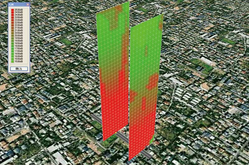
| Visualization by contours |
Visualization by contour lines |
Visualization with sphere shapes |
Simulation results can be checked from several view points. In addition
to by contours and contour lines, sound pressure level can be visualized
with grids or spheres.
- Development of parallelized algorithm perfect for the use of high-performance
computer
- Improvement of simulation result display
- Development of VR-Studio® noise simulation option
| ■ Noise measurement simulation service (option) |
|
This option can be selected as well as "High-performance computing
analysis and simulation service on noise". The noise in various construction
site and traffic is measured and the results are provided.
Actual measurment results combined with the visualization of the VR modeling
and the result of noise analysis simulation at the measurement site help
you to check the analysis result and make a comparative review.
|
Flow of the noise measurement simulation service |
High-performance computing
analysis and simulation service on noise |
|
1.
|
hear the overview of your request
via tel/email |
 |
| 2. |
Explain the estimation and working contents |
| |
| 3. |
-Create VR model of the measurement site
-Prediction analysis on noise when
sound resources are implemented |
|
 |
Noise measurement
simulation service (option) |
|
4. |
Measure noise at the site
|
| |
| 5. |
Create a report of the measurement result |
| |
| 6. |
Delivery
|
|
 |
|
 |
| Example of construction noise |
|
Example of road noise |
●Overview of the noise measurement simulation service
|
Noise measurement can be roughly divided into the following types, and
the "arbitrary measuring" is supported in this service. |
- Arbitrary measurement
Customized measurement that does not consider a specific standard
- Road noise measurement
Based on the "manual for the evaluation of environmental standard
related to noise II. Regional evaluation edition (region faced to roads)"
April 2000, Ministry of the Environment
- Construction noise measurement
Based on the "Guideline for the noise measurement of construction"
FY2009, Public Works Research Institute
●Types of general noise
|
manuals for evaluation and measurement are prepared for the following kinds
of noise. Inside the brackets are a name of each prediction model. |
- General environment noise
- Road traffic noise (ASJ RTN-Model2008)
- Noise by conventional lines
- Noise by Shinkansen lines
- Noise by airplane
- Construction noise (ASJ CN-Model2007)
|
In this service, the road traffic noise and construction noise are focused
on. |
●Measuring equipment
- Sound level meter: JIS C 1509-1
- Calibrator: JIS C 1515
- Level recorder: JIS C 1512 (planned)
- Data recorder: no JIS rule, support of 20Hz-10kHz (planned)
- Frequency analyzer: JIS C 1513 (planned)
|
|
| ■ Noise measurement simulation service: estimation example |
|
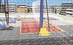
Case of construction noise |
●Noise analysis
|
For the status of the noise analysis (of construction noise), one sound
source is set at the upper side of the analysis range, and a wall of about
20 m length is set from the upper right to the left bottom, passing by
the sound source. The followings are the conditions. |
- Size of sound receiving area: 80 m x 80 m x 2 sides
- Sound source level: 112 dB
- Frequency of sound source: 1000 Hz
- Analytic elapsed time: 0.26 sec
- Intervals of analysis time: 0.01 sec
●Noise measurement
|
For the status of the noise measurement site (of construction noise), a
measurement case is assumed with four noise meters set around a construction
machine (object sound source, blue circle in the figure) and one day-of-year
noise meter set at the bottom of the drawing. |
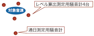 |
| Noise measurement (construction noise) |
|
|
| Conditions and estimate of noise analysis |
Conditions and estimate of noise measurement |
| Item |
Data |
| Fixed sound source |
1 |
| Moving sound source |
no |
| Sound receiver |
1 |
| Sound receive point |
289 |
Specified sound receive point
(the time series data to be organized) |
0 |
| Estimate |
¥269,646 |
|
| Item |
Data |
| Number of unit |
1 unit |
| Unit working cycle |
3 |
| Daily measurement point |
1 |
Moving vehicle noise
measurement point |
0 |
| Working time on the day |
9 hours |
| Estimate |
¥779,401 |
|
| *Tax is not included. |
 |
 |
| Noise analysis (construction noise) |
●Noise analysis
|
A vehicle is arranged at the center bottom of each two contour drawings
as a sound source.
The followings are the conditions. |
- Size of sound receiving area: 100 m x 400 m x 2 sides
- Sound source level: 100 dB
- Frequency of sound source: 85Hz
- Analytic elapsed time: 2.0 sec
- Intervals of analysis time: 0.02 sec
●Noise measurement
|
騒音測定(道路騒音)の現場状況としては、選択した道路断面(2ヶ所)の両側に測定用騒音計各1台設置し、断面を車両が通過する瞬間の音圧レベル分布を測定するケースを想定しました。 |
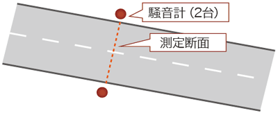 |
| Noise measurement (road noise) |
|
|
| Conditions and estimate of noise analysis |
Conditions and estimate of noise measurement |
| Item |
Data |
| Fixed sound source |
2 |
| Considering moving sound source |
no |
| Sound receiver |
2 |
| Sound receive point |
880 |
Specified sound receive point
(the time series data to be organized) |
0 |
| Estimate |
¥764,725 |
|
| Item |
Data |
| Section to measure |
1 |
| Measurement point |
2 |
| Traffic volume measurement |
yes |
| Traveling speed measurement |
yes |
| Noise measurement of hinterland |
no |
| Measuring time |
24 hours |
| Estimate |
¥2,681,066 |
|
| *Tax is not included. |
 |
 |
| Noise analysis (road noise) |
|
Case study of road noise analysis (Build Live Tokyo 2010) |
|
Simulation of road noise at residential area is under developing. Set a
vertical surface and a horizontal surface, and calculate a sound pressure
level at the time of a car passing by the center of the surfaces. The followings
are the conditions. |
- Size of sound receiving range: 40 m x 100 m x 2 sides
- Sound source level: 100 dB
- Frequency of sound source: 500Hz
- Analytic elapsed time: 0.2 sec
- Intervals of analysis time: 0.01 sec (analysis time by high-performance
computer: 9 min)
 |
 |
| Noise analysis (vertical) |
Noise analysis (horizontal) |
|
|
| ■ Tsunami and fluid analysis simulation service |
This service allows you to simulate the tsunami situation followed by a
mega-earthquake such as the Tohoku Earthquake happened in March 11, 2011
and then to obtain the result.
In this service, the simulation of tsunami followed by mega-earthquake
such as Nankai Trough earthquake is run via a tsunami analysis solver provided
by Prof. Fumihiko Imamura of Tohoku University. The situation from the
generation of tsunami to that the tsunami rushes toward the coast is simulated.
As the result of the simulation, how the tsunami rushes, the area which
has the highest tsunami and the time history of tsunami height at the chosen
area can be seen.
This simulation is run via Super Computer (FOCUS supercomputer) that FOCUS
(Foundation for Computational Science.) has. Making use of super computer
makes the calculation so fast even if it is large-scale computation.
 |
 |
Figure1 Analysis animation of Indian Ocean tsunami (2004)
(Tsunami research center in Tohoku University) |
| About the tsunami analysis solver |
The tsunami solver is based on the solver provided by Prof. Fumihiko Imamura of Tohoku University. This has the following features.
1. Propagation calculation of tsunami based on the shallow water long
wave theory
2. Analysis performed in a large-scale range via nesting method
3. Batch simulation from the tsunami generation to the propagation of an earthquake
4. The detailed representation of the coast area including the bank and river
1. Propagation calculation of tsunami based on the shallow water long wave theory
This solver is based on the theory called "shallow water long wave". Compared to deep-sea, the tsunami whose water depth is below 50m shows the characteristic behaviors, in which the wave height becomes higher etc. The shallow water long wave theory allows to represent the tsunami behavior along the coast in detail by taking into consideration a unique phenomenon for the tsunami propagation in a shallow area. The equation based on this shallow water long wave theory is calculated via finite difference method (FEM) on an orthogonal grid mesh.
2. Analysis performed in a large-scale range via nesting method
The propagation of tsunami sometimes reaches more than 100 km from the tsunami origin to the Japanese coast. However in case of calculating 100km square mesh, if selecting a small sized mesh to do a detailed analysis, simulation would be run at a distant time due to the vast number of mesh. On the other hand, selecting the large mesh can make the amount of calculation small and also make the simulation time shorter but make the detailed analysis more difficult.
The solver this time adopted the nesting method. Nesting method allows you to make the size of mesh in the coastal area where the damage caused by tsunami is expected to be huge more smaller, on the other hand, to make the size of mesh of the open sea more bigger and then let the small size mesh in the bigger sized mesh. Therefore this method makes it possible to run detail tsunami simulation by using the small size mesh in the coastal area without making the analysis region smaller. This also can shorten calculation time.
3. Batch simulation from the tsunami generation to the propagation of an earthquake
This solver allows you to calculate the initial wave height of tsunami from the faulting which causes an earthquake and calculate the propagation of tsunami based on the initial wave height.
Therefore the phenomenon of tsunami can be represented in more realistic way than setting the initial wave height which is virtual.
4. The detailed representation of the coast area including the bank and river
In this solver, the detailed simulation for the coastal area can be run by setting with or without a bank. Moreover taking into consideration a river can make it possible to represent river-runup of tsunami.
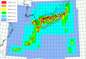
| The target analysis range |
In this service, the tsunami analysis is performed based on the earthquake
which was examined by the Committee for Modeling the Nankai Trough Megaquake
set up at the Cabinet Office, Government Of Japan.
The areas which can be analyzed in this service are the Pacific side of
sub-Ibaragi prefecture, Seto Inland Sea, the Sea of Japan side of Kyushu
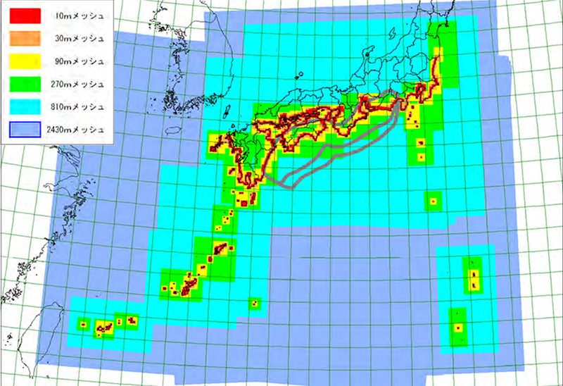
area and surrounding Okinawa. The whole of the area which can be analyzed
is shown in Figure 2. As for the areas shown in Figure 2, the following
terrain data of each mesh size has been prepared.
 |
|
|
10 m |
|
|
30 m |
|
|
90 m |
|
|
270 m |
|
|
810 m |
|
|
2,430 m |
|
| Figure2 The range which can be analyzed |
| Results obtained by this service |
The following results can be obtained by tsunami simulation in this service.
Animation showing how tsunami travels
Animation can show how tsunami travels from its generation at the earthquake occurrence area.
In so doing, the time when tsunami travels can be specified. Making use of UC-win/Road for playing the animation allows you to confirm the traveling tsunami from various kinds of angle of 360 degrees.
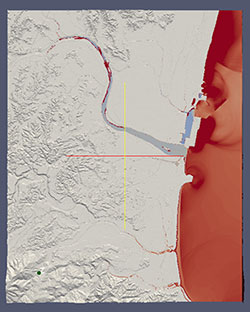 |
| Figure3 Analyzed exampe in Miyazaki area |
| Calculation via a super computer "Focus" |
Although the tsunami analysis solver used for this service adopt the method
called "Nesting" for shortening the calculation time, even so
the amount of calculation is likely to be huge. Therefore, "Focus
supercomputer" which is owned by Focus will be used to run simulation
in this service. In order to calculate via supercomputer, the parallel
processing via MPI is executed. It takes about more than 10 days for simulation
on general PC, while it takes about 5 days to calculate via Focus supercomputer.
*MPI (Message Passing Interface): Standard for parallel processing. It
is also possible to parallelize the several computers.
FORUM8 will move to more speeding up, stability and convenience. It will be expected to run the tsunami simulation with lower cost and in more user-friendly way to use.
 |
 |
 |
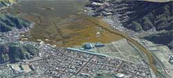
| Figure4 UC-win/Road Tsunami Simulation |
Referece (in Japanese)
-Japan Meteorological Agency: About Tsunami
http://www.jma.go.jp/jma/kishou/know/faq/faq26.html
-The Committee for Modeling the Nankai Trough Megaquake set up at the Cabinet Office, Government Of Japan
http://www.bousai.go.jp/jishin/nankai/model/
|
Report on the use of HPCI System for FORUM8's R&D project in FY 2013.
"Development of a rendering engine using The Supercomputer K" |
|
FORUM8 has carried out its trial and the main R&D project as its attempt to be
selected as the applicant to whom the privilege to use K in the R&D will be granted, during the following periods.
・Trial (project number: hp130034): 2013/05/17 - 2013/11/16
Project name: "Development of a high-speed rendering environment that uses photo-realistic
engine"
・Main
R&D project carried out for a possible selection as the project in
which K is to be adopted (project number : hp130093): 2013/10/01 - 2014/03/31
The outcome of the above is as the follows.
|
| |
2) Trial (project number: hp130034): 2013/05/17 - 2013/11/16 |
The
trial has been carried out with the objective of verifying whether
LuxRender, a rendering engine of an open source, operates in K.
In FOCUS, the operation of LuxRender has already been realized, and an
operation of about 30 nodes has been verified. The number of nodes in K is
about 80,000, which is
enormous, and the supercomputer is in an environment where
it is possible to verify up to how much the processes can be sped
up, but in the trial, the operation of LuxRender itself and
parallel computing using a small number of nodes without communication
was first carried out. In the environment we built for the last trial test, an environment for creating an animation by LuxRender has been constructed, which
could not be realized in FOCUS due to the insufficient number of nodes.
2-1) Porting of LuxRender in K
In K, compilation by a compiler made by Fujitsu was the
standard, but when it comes to an open source software rendering system
such as LuxRender, compilation via gcc, cmake, etc. is required. Also,
the use of SSE command was not possible as the supercomputer had sparc
CPU instead of an Intel CPU.
First, an investigation to find out whether compiling is possible by
cmake, gcc, etc. was made, and a compiling environment was created by
installing
tools on FORUM8's own terms for the parts that could not be compiled.
Next, by
creating a library which emulates SSE command and installing it into
LuxRender, the compilation of LuxRender finally succeeded.
2-2) Parallelization without communication
LuxRender has a mechanism of performing parallel computing by socket communication, but
it turns out that K does not have any empty socket that can be used
because communication needs to be done by MPI. Therefore, an algorithm
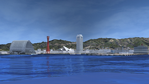
which can perform parallel computing by dividing the image was developed. Diagram A is an
image produced by parallel computing via image division.
 |
| Figure A : Rendering result (bath) |
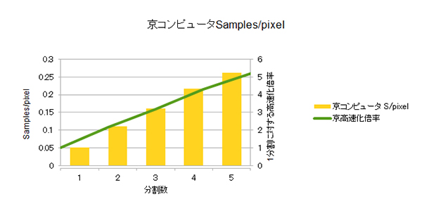 |
| Figure B : S/pixel regarding the division numbers |
The
processing speed for each division number is shown in Figure B.
Samples/pixel shows the sampling numbers per pixel. Although a linear
speed-up, the image quality decreases when the division number reaches
the limit of about 30, nevertheless, this is a good result for the kind
of result that can be obtained from a verfication of an acceleration
algorithm.
2-3) Construction of an environment for animation rendering via LuxRender
A rendering of an animation was carried out by creating an environment
for rendering via highly parallel computing in K an animation exported in LuxRender format by Blender.
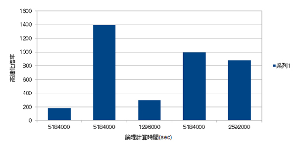 |
| Figure C : Acceleration rate of the speed of rendering a sample scene |
Figure C shows the extent to which the speed of rendering an animation scene created as a sample can
increase when it is rendered by K. The horizontal axis is the time it
takes if the animation is rendered in 1 node, and the vertical axis is
the number of times the rendering speed will increase when highly
parallel computing is done by K.
In
the case K is assigned with an execution, there maybe some waiting time
before execution depending on the availability. Since the assumption
here is that K is put to actual use, the length of time it takes to
obtain the results from the start of the execution has been
measured. The result was that the speed can be
expected to increase by about 1400 times compared to an ordinary
PC, without waiting time.
|
|
3)
Main R&D project carried out for a possible selection as the
project in which K is to be adopted (task number : hp130093) 2013/10/01
- 2014/03/31 |
In
the main R&D project, we did a test to see how fast a still image
can be rendered by K performing parallel computing on about 10,000
nodes.
LuxRender is structured so that it can scatter light rays among nodes during parallel computing in network mode. However,
since K cannot use sockets for communication among nodes, communication must be done through MPI, which makes it necessary to
add codes substantially.
Also, as more nodes need to communicate among each other in the case of highly parallel computing,
the overall communication volume will inevitably increase, causing
speed to slow down encountering a situation where increasing nodes
doesn't increase speed, but measures have
been taken to solve this problem (parallelization of I/O).
3-1) High parallel computing on still images via communications through MPI
Communication between nodes were done by socket communication, but by newly
creating an emulatation library based on MPI, the method of communication could be replaced
to a communication via MPI. The result being K can can now render still images by highly parallel computing.
 |
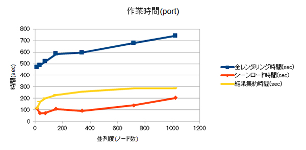
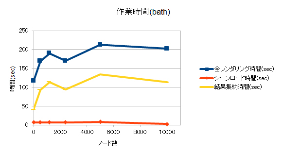
| Figure D : Rendering result (port) |
 |
| Figure
E : Overall processing time required in parallel computing via MPI
communication, which varies according to the number of nodes to be used
for parallel computing. |
The
overall rendering time is the length of time from when rendering begins
to when the result is obtained, the scene loading time is the time
required for all nodes to finish loading the scene, and the result
aggregation time is the time required to create one image by collecting
the result from each node. The actual rendering time per node is 4
minutes, so the ratio of incidental processing (scene loading time and result aggregation time) to overall rendering time seems large, but increasing the rendering time per node does
not change the incidental processing time. Furthermore, the value which represents
the overall amount of data that can be rendered (amount
of data rendered per pixel ( Samples/pixel)) will increase if the
number of nodes to be used for parallel computing increases.
The
graph in Figure E shows nodes of up to 1,000 along the x-axis.
According to the result, the processing time increases according to the
number of nodes, and when the number of nodes surpassed the value of approximately 1000, the system hung up
and stopped.
3-2) Parallelization of I/O
The hang up is caused by a failure to access a file in NFS due to a program of 1000 nodes all trying to access the file at one
time. So it has been
decided to use the mechanism of distributing files among a number of
nodes, a mechanism
equipped in K. By storing files on a number of nodes in advance, each
node will access the files stored in its own node, the result being
rendering is no longer interrupted by a hang. The
other issue relates to the time required to integrate the result rendered by each node into one image when nodes are in great number.
For instance, in the case of 10,000
nodes, even if rendering takes only one minute for each node, the
entire process up to the image completion would take 10,000 minutes,
which is too long for anyone to wait. To solve this problem, a measure
which aggregates the result
images per adjacent nodes and programs an algorithm which aggregates
all the images into one image in the end was taken.
The measure proved to be very effective as the time required to
aggregate the images was reduced from O (number of nodes) to O
(log2(number of nodes)). Also,
parallel computating has been carried out to every part including the
part
where status communication, etc. were previously not done through
parallel computing.
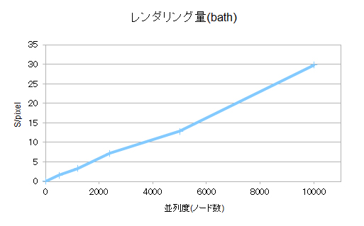 |
| Figure F: Amount of data that can be rendered through parallel I/O as a
function of node quantity. |
Figure F is a graph illustrating the amount of data that can be rendered
as a function of node quantity after employing parallel I/O. It was confirmed
that the speed improves linearly as you increase the number of nodes, until
it reaches 10,000 nodes.
 |
| Figure G : The working time as a function of node quantity after employing parallel I/O |
Figure G is a graph illustrating the working time as a function of node quantity after employing parallel I/O.
Since the rendering time per node is only one minute, the ratio of
incidental processing to overall rendering time is large, but
increasing the rendering time per node would not make any difference.
At first it gradually becomes slower, but the speed becomes flat from
the point where the node quantity goes above 1000, and the processing
time remains the same until 10,000 nodes. |
| The
next step is to increase stability. Optimization has not been carried
out yet, hence the need to improve speed. In diagram G, the time spent
on aggregating the results is quite long, therefore there is
plenty of room for improvement in the time. |
|
| Scheduled high-performance computing service |
|
Under development |
|
Ground energy simulation "GeoEnergy"
- Large-scaled Tsunami and fluid analysis service
3DVR cloud "VR-Cloud® seivice"
- High amount of calculation and data transition by the cooperation between
cloud and high performance computer
|
|